Save plot animations as video in Python

For time-resolved simulations, you may want to save a dynamic (animated) plot as a video so that it can be played back in sync with other simulation variables. This guide describes how to accomplish this with the “double pendulum simulation” as an example.

Nominal has 1st class support for video ingestion, analysis, time sychronization across sensor channels, and automated checks that signal when a video feature is out-of-spec.

This guide demonstrates how to upload a video file to Nominal in Python. Other guides in the Video section demonstrate basic Python video analysis and computer vision for video pre-processing prior to Nominal upload.

Double pendulum simulation

The double pendulum consists of two pendulums attached end to end, where the motion of one pendulum influences the other, creating complex, chaotic dynamics. It is a classic problem in physics that demonstrates how even simple systems can exhibit unpredictable behavior due to sensitivity to initial conditions.

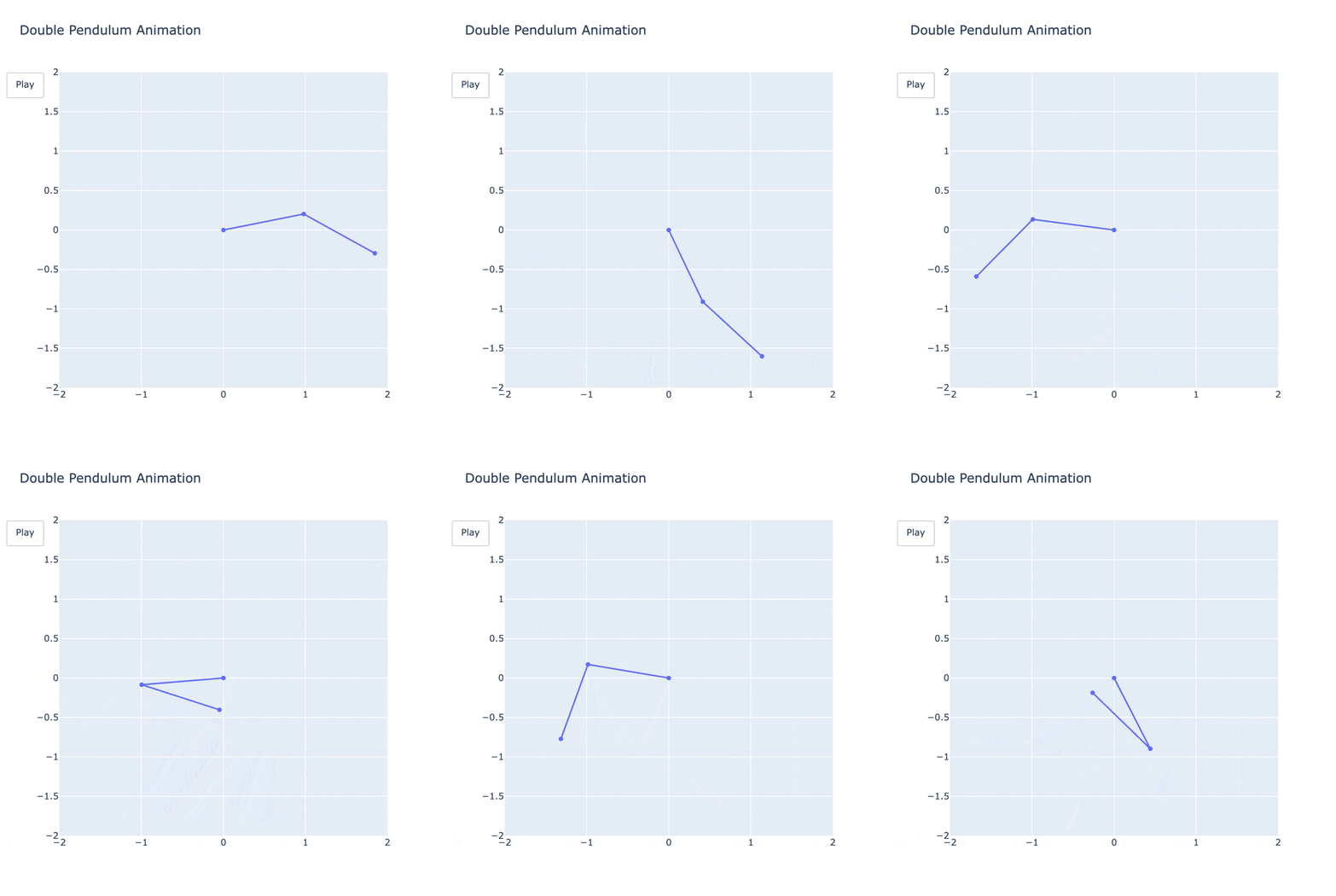
If you’ve never seen the double pendulum simulation, below is a time-resolved animation of its solution. Note that the simulation length is 25 seconds.
1import numpy as np
2import plotly.graph_objs as go
3from scipy.integrate import solve_ivp
4
5# Parameters for the double pendulum
6m1, m2 = 1.0, 1.0 # masses of the pendulums
7L1, L2 = 1.0, 1.0 # lengths of the pendulums
8g = 9.81 # gravitational acceleration
9
10# Equations of motion for the double pendulum
11def double_pendulum_equations(t, y):
12 theta1, z1, theta2, z2 = y
13 delta = theta2 - theta1
14
15 # Equations of motion
16 den1 = (m1 + m2) * L1 - m2 * L1 * np.cos(delta) * np.cos(delta)
17 den2 = (L2 / L1) * den1
18
19 dydt = [
20 z1,
21 (m2 * L1 * z1 * z1 * np.sin(delta) * np.cos(delta) +
22 m2 * g * np.sin(theta2) * np.cos(delta) +
23 m2 * L2 * z2 * z2 * np.sin(delta) -
24 (m1 + m2) * g * np.sin(theta1)) / den1,
25 z2,
26 (- m2 * L2 * z2 * z2 * np.sin(delta) * np.cos(delta) +
27 (m1 + m2) * (g * np.sin(theta1) * np.cos(delta) -
28 L1 * z1 * z1 * np.sin(delta) -
29 g * np.sin(theta2))) / den2
30 ]
31 return dydt
32
33# Initial conditions and time span
34y0 = [np.pi / 2, 0, np.pi / 2, 0] # initial angles and angular velocities
35t_span = (0, 25)
36t_eval = np.linspace(*t_span, 500)
37
38# Solve the equations
39solution = solve_ivp(double_pendulum_equations, t_span, y0, t_eval=t_eval, method='RK45')
40theta1, theta2 = solution.y[0], solution.y[2]
41
42# Calculate positions of the pendulums
43x1 = L1 * np.sin(theta1)
44y1 = -L1 * np.cos(theta1)
45x2 = x1 + L2 * np.sin(theta2)
46y2 = y1 - L2 * np.cos(theta2)
47
48# Create animation using plotly
49frames = []
50for i in range(len(t_eval)):
51 frames.append(go.Frame(data=[
52 go.Scatter(x=[0, x1[i], x2[i]], y=[0, y1[i], y2[i]], mode="lines+markers")
53 ]))
54
55# Set up the initial plot
56fig = go.Figure(
57 data=[go.Scatter(x=[0, x1[0], x2[0]], y=[0, y1[0], y2[0]], mode="lines+markers")],
58 layout=go.Layout(
59 title="Double Pendulum Animation",
60 xaxis=dict(range=[-2, 2], zeroline=False),
61 yaxis=dict(range=[-2, 2], zeroline=False),
62 updatemenus=[dict(type="buttons", showactive=False, buttons=[dict(label="Play",
63 method="animate",
64 args=[None, {"frame": {"duration": 50, "redraw": True},
65 "fromcurrent": True}])])],
66 width=600,
67 height=600
68 ),
69 frames=frames
70)
71
72# Show the animation
73fig.show()

double-pendulum

Convert animation to video

To convert the Plotly animation to a video, we’ll install the imagio library with the ffmpeg plugin:

pip3 install imageio[ffmpeg]

Prior to running the above command, you’ll also want to install the underlying ffmpeg library. On a Mac you can install this with brew install ffmpeg. For installation instructions for other operating systems, please see the official FFmpeg download page.

For more information about this plugin, please refer to the imageio docs.

Now, we’ll modify the simulation code above to to save an image for each animation frame with Plotly’s write_image() function. At the end of the simulation, we’ll stitch these images together into a video with imageio’s get_writer() function.

1import os
2import numpy as np
3import plotly.graph_objs as go
4from scipy.integrate import solve_ivp
5import imageio.v2 as imageio
6
7# Parameters for the double pendulum
8m1, m2 = 1.0, 1.0
9L1, L2 = 1.0, 1.0
10g = 9.81
11
12# Equations of motion
13def double_pendulum_equations(t, y):
14 theta1, z1, theta2, z2 = y
15 delta = theta2 - theta1
16
17 den1 = (m1 + m2) * L1 - m2 * L1 * np.cos(delta) ** 2
18 den2 = (L2 / L1) * den1
19
20 dydt = [
21 z1,
22 (m2 * L1 * z1 ** 2 * np.sin(delta) * np.cos(delta) +
23 m2 * g * np.sin(theta2) * np.cos(delta) +
24 m2 * L2 * z2 ** 2 * np.sin(delta) -
25 (m1 + m2) * g * np.sin(theta1)) / den1,
26 z2,
27 (- m2 * L2 * z2 ** 2 * np.sin(delta) * np.cos(delta) +
28 (m1 + m2) * (g * np.sin(theta1) * np.cos(delta) -
29 L1 * z1 ** 2 * np.sin(delta) -
30 g * np.sin(theta2))) / den2
31 ]
32 return dydt
33
34# Initial conditions and time span
35y0 = [np.pi / 2, 0, np.pi / 2, 0]
36t_span = (0, 25)
37t_eval = np.linspace(*t_span, 500)
38
39# Solve the equations
40solution = solve_ivp(double_pendulum_equations, t_span, y0, t_eval=t_eval, method='RK45')
41theta1, theta2 = solution.y[0], solution.y[2]
42
43# Calculate positions
44x1 = L1 * np.sin(theta1)
45y1 = -L1 * np.cos(theta1)
46x2 = x1 + L2 * np.sin(theta2)
47y2 = y1 - L2 * np.cos(theta2)
48
49# Save frames as images
50filenames = []
51for i in range(len(t_eval)):
52 fig = go.Figure(
53 data=[go.Scatter(x=[0, x1[i], x2[i]], y=[0, y1[i], y2[i]], mode="lines+markers")],
54 layout=go.Layout(
55 title="Double Pendulum Animation",
56 xaxis=dict(range=[-2, 2], zeroline=False),
57 yaxis=dict(range=[-2, 2], zeroline=False),
58 width=600,
59 height=600
60 )
61 )
62 filename = f'frame_{i:03d}.png'
63 fig.write_image(filename)
64 filenames.append(filename)
65
66# Create video from frames using imageio
67with imageio.get_writer('double_pendulum.mp4', fps=20) as writer:
68 for filename in filenames:
69 image = imageio.imread(filename)
70 writer.append_data(image)
71
72# Cleanup
73for filename in filenames:
74 os.remove(filename)
75
76print("Video saved as 'double_pendulum.mp4'")

Note that the simulation video has been saved to double_pendulum.mp4.

Display video inline

If you’re working in Jupyter notebook, here’s a shortcut to display the video inline in your notebook.

1from ipywidgets import Video
2Video.from_file(video_path)

Save simulation channels

We’ll run the same simulation a final time to extract channels such as the pendulum fulcrum’s heights, momentums, PEs and KEs, etc.

Simulations are often time-consuming to run. In practice, you would want to extract the simulation result, video frames, and important channel values in a single pass. For the pedagogical purposes of this tutorial, however, we’ve separated the extraction of these 3 artifacts into 3 identical but separate simulation runs.
1import numpy as np
2import pandas as pd
3from scipy.integrate import solve_ivp
4from datetime import datetime, timedelta
5
6# Parameters for the double pendulum
7m1, m2 = 1.0, 1.0 # masses of the pendulums
8L1, L2 = 1.0, 1.0 # lengths of the pendulums
9g = 9.81 # gravitational acceleration
10
11# Equations of motion for the double pendulum
12def double_pendulum_equations(t, y):
13 theta1, z1, theta2, z2 = y
14 delta = theta2 - theta1
15
16 # Equations of motion
17 den1 = (m1 + m2) * L1 - m2 * L1 * np.cos(delta) * np.cos(delta)
18 den2 = (L2 / L1) * den1
19
20 dydt = [
21 z1,
22 (m2 * L1 * z1 * z1 * np.sin(delta) * np.cos(delta) +
23 m2 * g * np.sin(theta2) * np.cos(delta) +
24 m2 * L2 * z2 * z2 * np.sin(delta) -
25 (m1 + m2) * g * np.sin(theta1)) / den1,
26 z2,
27 (- m2 * L2 * z2 * z2 * np.sin(delta) * np.cos(delta) +
28 (m1 + m2) * (g * np.sin(theta1) * np.cos(delta) -
29 L1 * z1 * z1 * np.sin(delta) -
30 g * np.sin(theta2))) / den2
31 ]
32 return dydt
33
34# Initial conditions and time span
35y0 = [np.pi / 2, 0, np.pi / 2, 0] # initial angles and angular velocities
36t_span = (0, 25)
37t_eval = np.linspace(*t_span, 500)
38
39# Solve the equations
40solution = solve_ivp(double_pendulum_equations, t_span, y0, t_eval=t_eval, method='RK45')
41theta1, theta2 = solution.y[0], solution.y[2]
42
43# Calculate positions, velocities, accelerations, and energies
44x1 = L1 * np.sin(theta1)
45y1 = -L1 * np.cos(theta1)
46x2 = x1 + L2 * np.sin(theta2)
47y2 = y1 - L2 * np.cos(theta2)
48
49vx1 = np.gradient(x1, t_eval)
50vy1 = np.gradient(y1, t_eval)
51vx2 = np.gradient(x2, t_eval)
52vy2 = np.gradient(y2, t_eval)
53
54ax1 = np.gradient(vx1, t_eval)
55ay1 = np.gradient(vy1, t_eval)
56ax2 = np.gradient(vx2, t_eval)
57ay2 = np.gradient(vy2, t_eval)
58
59momentum_1_x = m1 * vx1
60momentum_1_y = m1 * vy1
61momentum_2_x = m2 * vx2
62momentum_2_y = m2 * vy2
63
64height_1 = y1 + L1 + L2
65height_2 = y2 + L1 + L2
66
67kinetic_energy_1 = 0.5 * m1 * (vx1**2 + vy1**2)
68kinetic_energy_2 = 0.5 * m2 * (vx2**2 + vy2**2)
69
70potential_energy_1 = m1 * g * (y1 + L1 + L2)
71potential_energy_2 = m2 * g * (y2 + L1 + L2)
72
73# Generate ISO8601 formatted timestamps
74start_time = datetime.now()
75absolute_time = [start_time + timedelta(seconds=t) for t in t_eval]
76
77# Create DataFrame with full header names
78data = {
79 "Timestamp (ISO8601)": [t.isoformat() for t in absolute_time],
80 "Momentum 1 (X)": momentum_1_x, "Momentum 1 (Y)": momentum_1_y,
81 "Momentum 2 (X)": momentum_2_x, "Momentum 2 (Y)": momentum_2_y,
82 "Acceleration 1 (X)": ax1, "Acceleration 1 (Y)": ay1,
83 "Acceleration 2 (X)": ax2, "Acceleration 2 (Y)": ay2,
84 "Velocity 1 (X)": vx1, "Velocity 1 (Y)": vy1,
85 "Velocity 2 (X)": vx2, "Velocity 2 (Y)": vy2,
86 "Height 1": height_1, "Height 2": height_2,
87 "Kinetic Energy 1": kinetic_energy_1, "Kinetic Energy 2": kinetic_energy_2,
88 "Potential Energy 1": potential_energy_1, "Potential Energy 2": potential_energy_2
89}
90
91df = pd.DataFrame(data)
92
93# Save the DataFrame to a CSV file
94csv_file_path_full_headers = "double_pendulum_full_headers.csv"
95df.to_csv(csv_file_path_full_headers, index=False)
96
97df

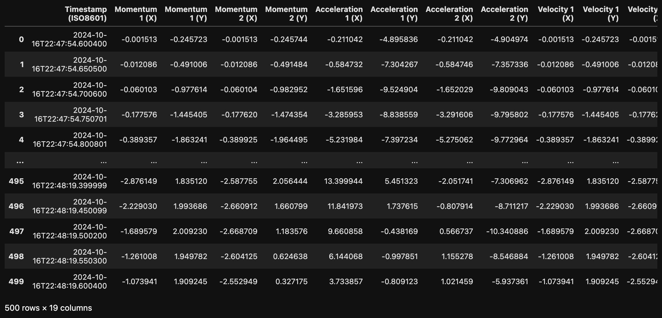
simulation-dataframe

Note that we saved the channel data in a CSV file - double_pendulum_full_headers.csv.

Finally, let’s upload these channels and video to Nominal so that we can visualize them together.

Connect to Nominal

Get your Nominal API token from your User settings page.

See the Quickstart for more details on connecting to Nominal from Python.

1import nominal.nominal as nm
2
3nm.set_token(
4 base_url = 'https://api.gov.nominal.io/api',
5 token = '* * *' # Replace with your Access Token from
6 # https://app.gov.nominal.io/settings/user?tab=tokens
7)
If you’re not sure whether your company has a Nominal tenant, please reach out to us.

Create a Run

First, we’ll create a Run to which we’ll attach our video and channel data.

In Nominal, Runs are containers of multimodal test data - including Datasets, Videos, Logs, and database connections.

To see your organization’s latest Runs, head over to the Runs page

1import nominal.nominal as nm
2
3sim_run = nm.create_run_csv(
4 file = "double_pendulum_full_headers.csv",
5 name = "double_pendulum_run",
6 timestamp_column = "Timestamp (ISO8601)",
7 timestamp_type = "iso_8601",
8)

Note that create_run_csv() automatically adds the CSV file to the Run and sets the Run’s start and end time.

Add Video to Run

Nominal Video uploads need an absolute start time. We’ll grab this start time from the channel dataframe:

1ts_start = df['Timestamp (ISO8601)'][0]
2ts_start

2024-10-16T22:47:54.600400

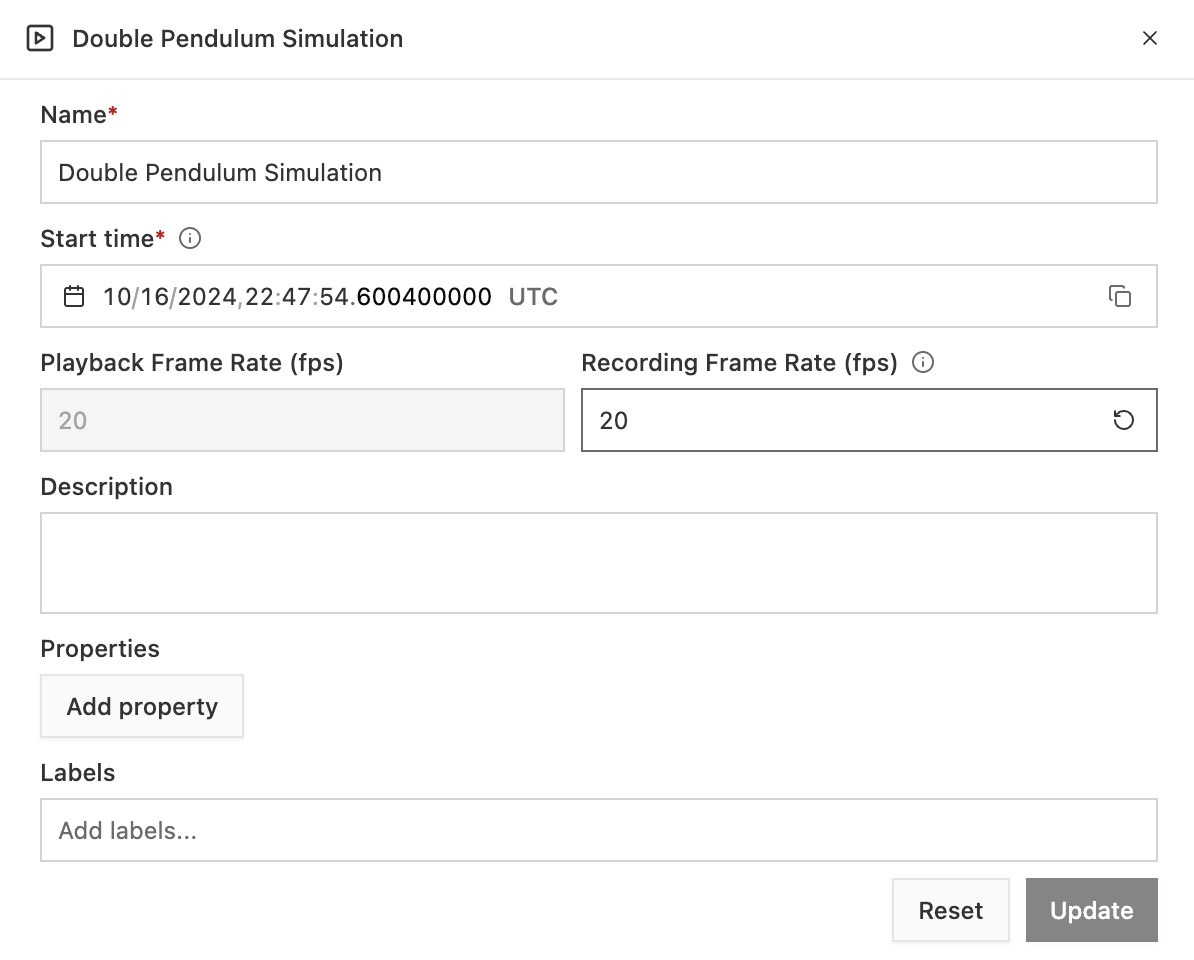
Adjust Video Start

Nominal has many tools to precisely sync video playback with channel data that was either extracted from the video or recorded independently at the same time as the video.

If you select a video on the video datasets page (login required), then you can adjust video metadata such as it start timestamp.
video-start-date

Create a Workbook

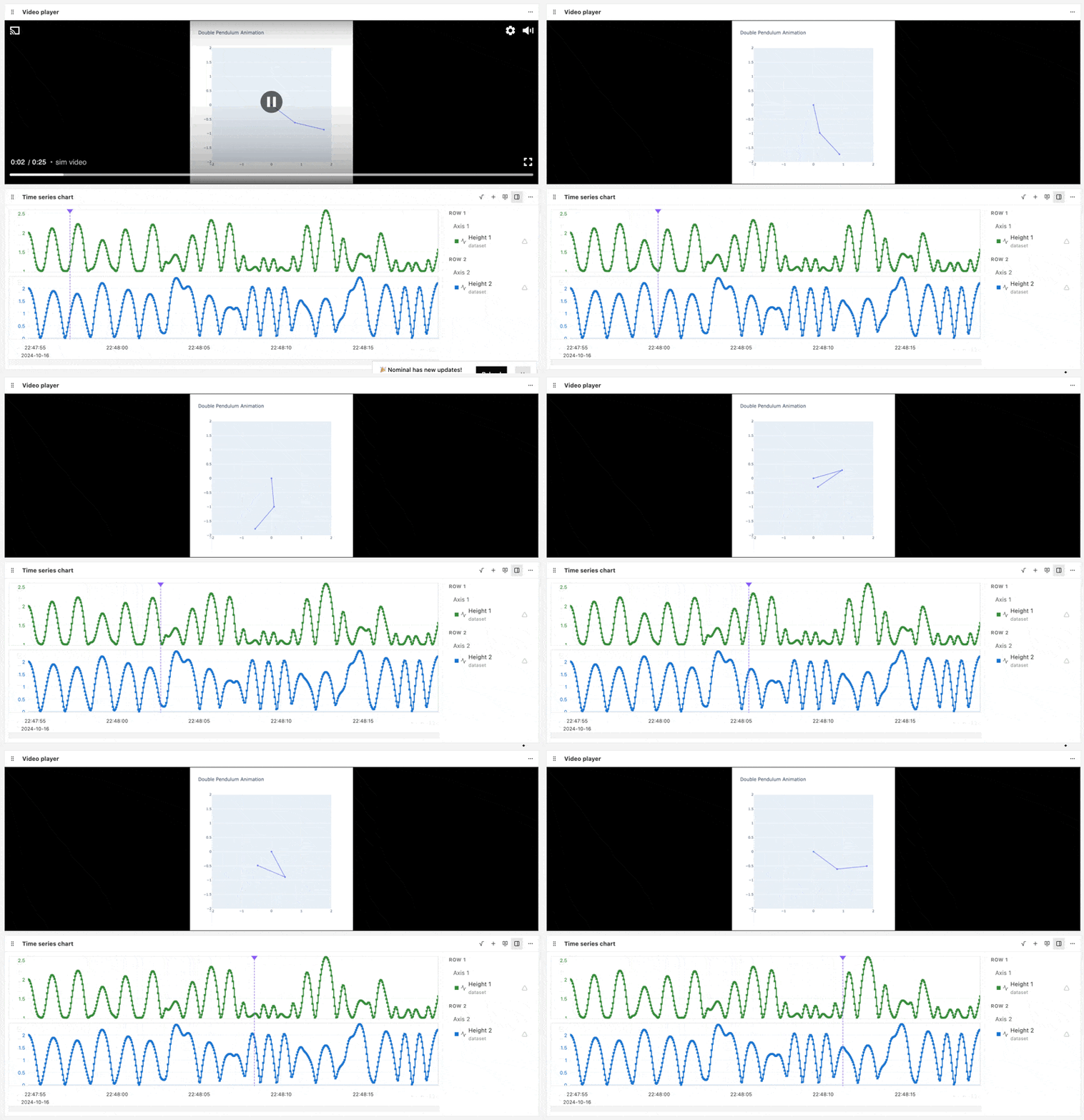
Our simulation video and channel data is now uploaded on the Nominal platform, where it can be collaboratively analyzed and benchmarked against real-world data.

Below is an example Nominal Workbook that syncs the pendulum fulcrum heights with the pendulum simulation video playback:
simulation-workbook

Other channels such as pendulum fulcrum momentum, acceleration, and kinetic energy can also be plotted. Workbook transforms and formulas can be used to calculate derived channels such as the RMS acceleration.

As an exercise, consider solving the simulation with a different ODE solver and comparing the results in a Nominal Workbook.